(→Sub-module for asymptotic modeling of Flame-Balls) |
(→The FLAMEX Solver) |
||
| Line 1: | Line 1: | ||
==The FLAMEX Solver== | ==The FLAMEX Solver== | ||
| − | |||
[[File:Flamex.jpg|240px]] | [[File:Flamex.jpg|240px]] | ||
| − | |||
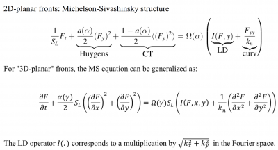
FLAMEX is a suite of solvers able to compute high accuracy solutions to non-linear non-local asymptotics-based evolution equations (EE), of 1rt | FLAMEX is a suite of solvers able to compute high accuracy solutions to non-linear non-local asymptotics-based evolution equations (EE), of 1rt | ||
For propagatong fronts, the EEM (Evolution Equation Modeling) can be found by solving exactly the set of | For propagatong fronts, the EEM (Evolution Equation Modeling) can be found by solving exactly the set of | ||
| Line 9: | Line 7: | ||
* the local kinematic relation defining the local front velocity (e.g. with respect to local curvature). | * the local kinematic relation defining the local front velocity (e.g. with respect to local curvature). | ||
when the density contrast between 'hot' and 'cold' fluids is asymptotically small. | when the density contrast between 'hot' and 'cold' fluids is asymptotically small. | ||
| − | |||
| − | |||
{| class="wikitable" | {| class="wikitable" | ||
|+ Examples of first-order in time obtained EEM: for 2D planar, 3D planar, or 3D expanding fronts | |+ Examples of first-order in time obtained EEM: for 2D planar, 3D planar, or 3D expanding fronts | ||
| Line 16: | Line 12: | ||
|[[File:OUIEqEEM_1D.png|400 px]] | |[[File:OUIEqEEM_1D.png|400 px]] | ||
|} | |} | ||
| − | |||
| − | |||
| − | |||
== Main features== | == Main features== | ||
Revision as of 11:38, 1 April 2016
Contents
The FLAMEX Solver
 FLAMEX is a suite of solvers able to compute high accuracy solutions to non-linear non-local asymptotics-based evolution equations (EE), of 1rt
For propagatong fronts, the EEM (Evolution Equation Modeling) can be found by solving exactly the set of
- Euler equations
- Rankine-Hugoniot jump relations
- the local kinematic relation defining the local front velocity (e.g. with respect to local curvature).
when the density contrast between 'hot' and 'cold' fluids is asymptotically small.
|

|
Main features
- Solving first-order or second order EE in the Fourier or Fourier-Legendre basis.
- Time resolution using ETDRK1 and 4, using contour integrals to avoid cancelation errors (Trefethen et al. 2005)
- EEM for 2D or 3D planar, 3D expanding/converging fronts, acoustics, fast-transients..
- Laminar or turbulent configurations (EE with additive noise, e.g. Passot-Pouquet, Kraichnan-Celik, Von Karman/Pao or 'DNS turbulence')
Sample Results
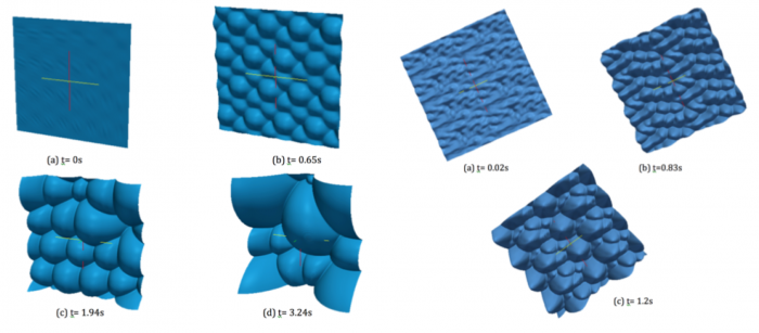
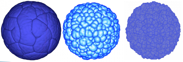
We show below a short gallery of pictures obtained using the FLAMEX solver.
|
|
Notice the 'soccer-ball' and 'cauliflower' aspects of the front, as described by Zel'dovitch in the 40's.
- See also some quantitative comparisons between FLAMEX and DNS (HALLEGRO) results at [1]
- More details (and comparisons with experimental results) in [2], [3]
Sub-module for asymptotic modeling of Flame-Balls
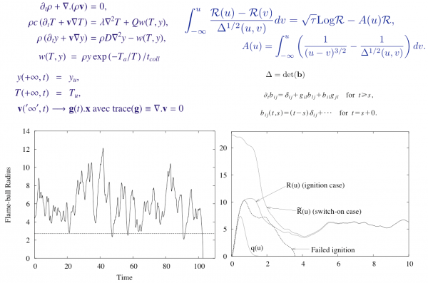
A sub-module of FLAMEX has also been devoted to the numerical solution to flame-balls (FB) dynamics. Using a Batchelor approximation for the surrounding Lagrangian flow and high activation energy asymptotics, we derived a nonlinear forced (stochastic) integrodifferential equation for the current FB radius. This gives access to the FB response to the ambiant Lagrangian rate-of-strain tensor g(t). For a diagonal g(t) deduced from random Markov processes of the Ornstein- Uhlenbeck type, or linearly filtered versions thereof, extensive numerical simulations and approximate theoretical analyses agree that
- flame balls can definitely live for much longer than their time of spontaneous expansion/collapse;
- large enough values of t_life are compatible with Poisson statistics;
- the variations of with the characteristics of g(t) mirror the latter’s statistics, more precisely that of trace(g*g).
|
Participants
Yves D'Angelo, Guy Joulin, Eric Albin, Rui Rego, Gaël Boury, Lancelot Boulet, Viphaphorn Srinavawongs, Yosifumi Tsuji.